Obsolete, see A New Wood Light Standardization Idea with No Vanila Disparity instead.
In this discord post I suggested a wood light ‘standardization’ solution, which summarizes to gradually speed up time after the game detects the portal being built. While I claim it is a much more elegant solution than directly forcing a light after a given amount of time, I did not mention how much time should be accelerated over time and how exactly this will hopefully preserve as much properties of unstandardized wood light as possible while reduce as much luck factor as possible. In this thread, I will dive into:
- properties of unstandardized wood light that we would like to preserve
- modeling different standardization solutions & how to measure how good they are
- some good example solutions
¹ The process that flammable blocks catch fire from lava is called Fire Spread in the wiki, but it is both unintuitive and easily confused with the process flammable blocks catch fire from another fire, which works fundamentally different. In the discord post I got that wrong but I stand by my term and in this post I am going to call it Fire Generation.
0. Preparation
From the video for wood light setup we all know and love
New Fastest Woodlight Design (afaik)
I found the code used for simulating wood light:
Flintless-simulator: Simulates flintless nether portal lighting
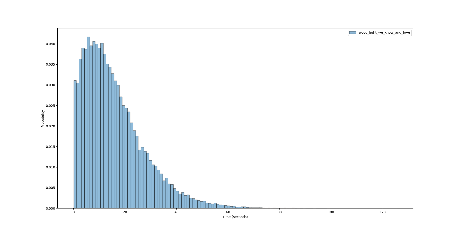
In the demo there isn’t actually nbt file and data for the pncakespoon setup, so I quickly pluged in the setup to generate the data. The results are as follows:
Avg light time: 15.914893000000001 +- 0.053752092172965886 ,
std: 12.01933320315861 , sample size: 50000
Failure rate: 0.0
(Original code used KDE to generate a smoothed distribution, but it is slightly bugged because it showed distorted probabilities at time = 0:
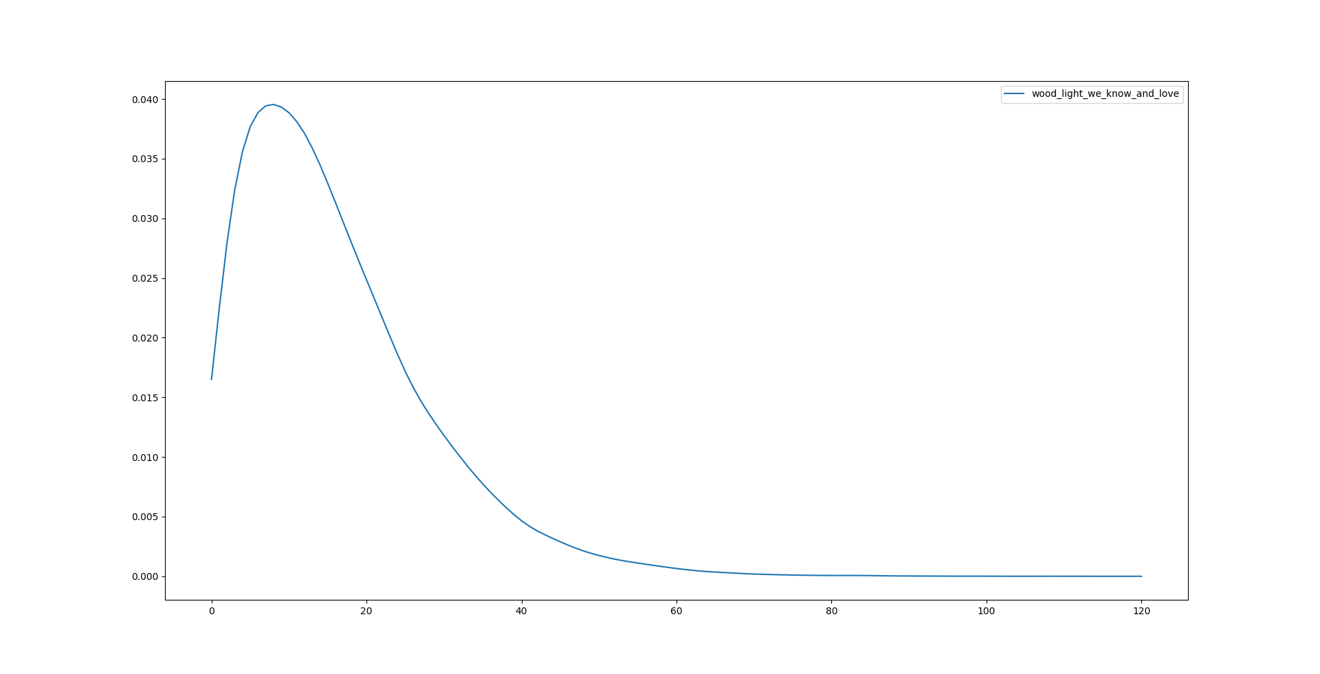
Here I went on a different approach of approximation with a model combining 3 arctan functions as the hazard function:
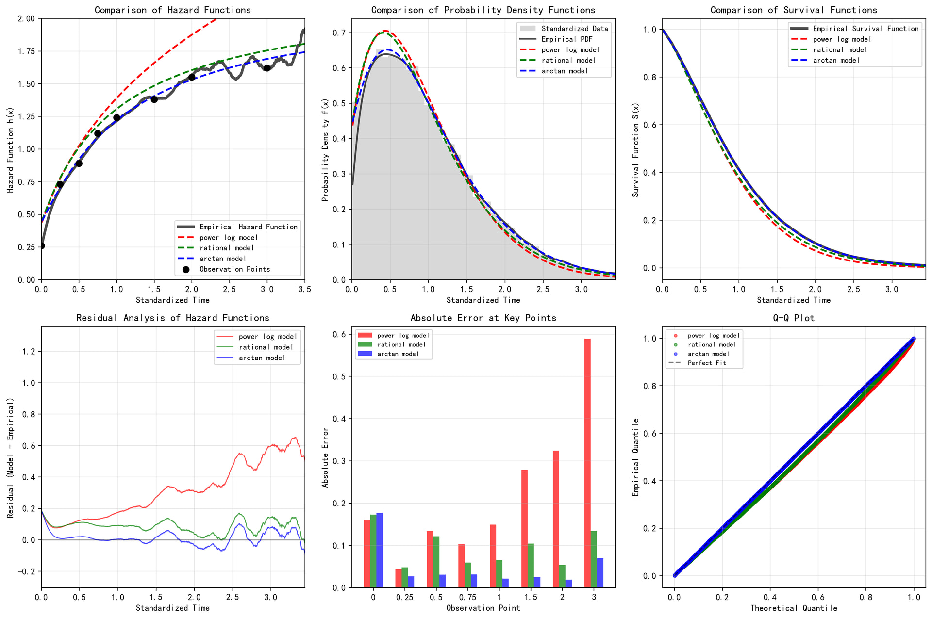
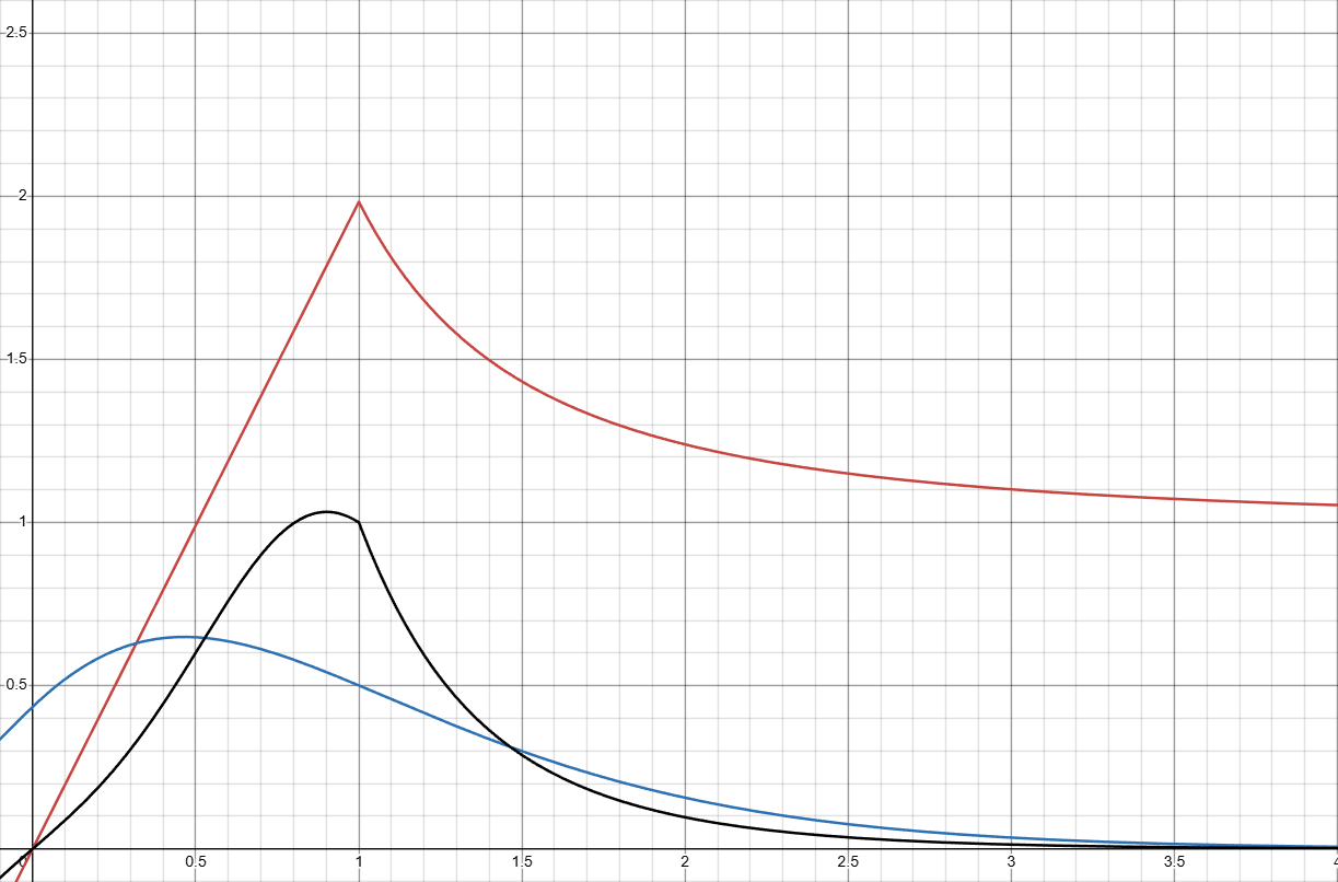
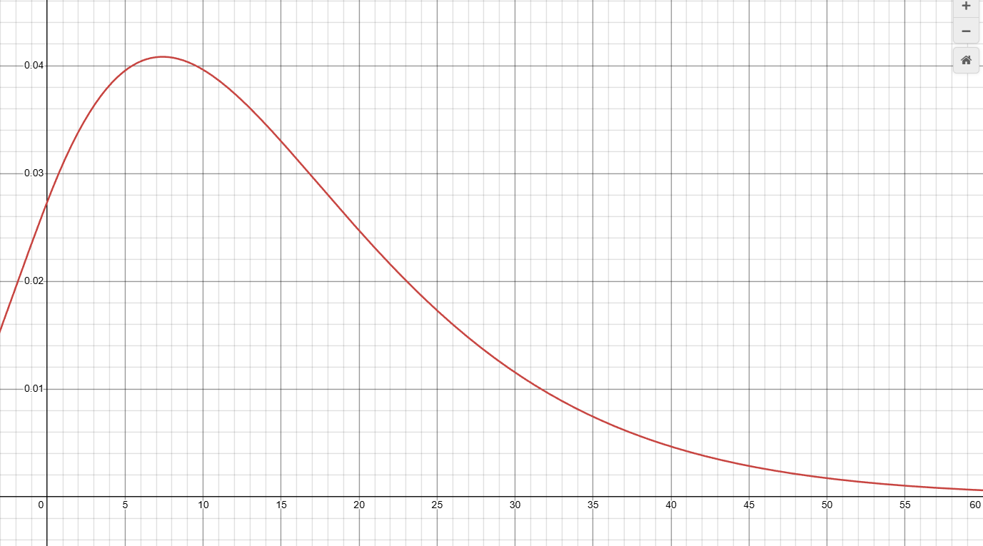
Original PDF f_o(x):
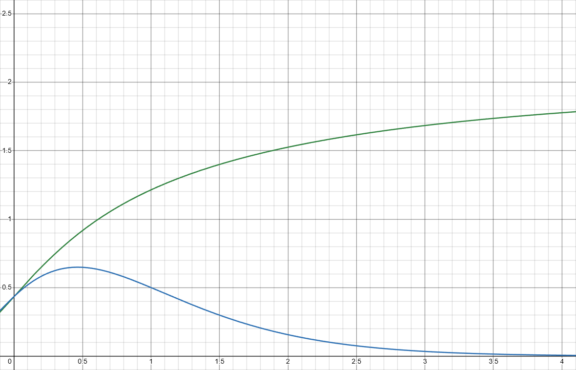
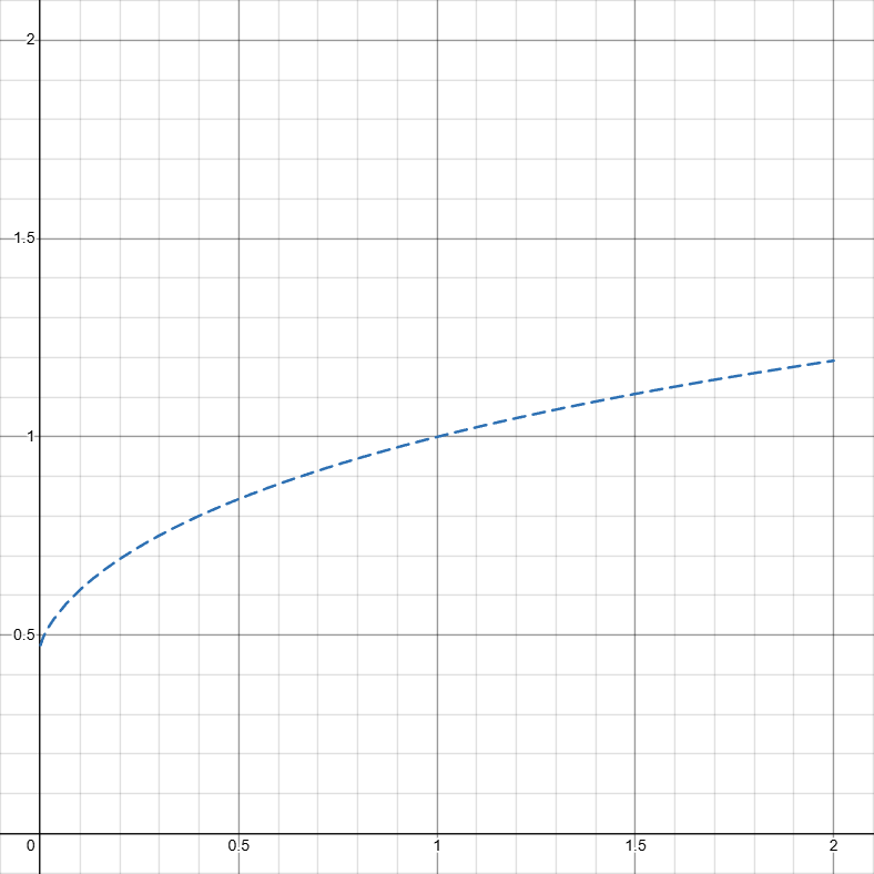
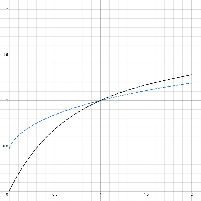
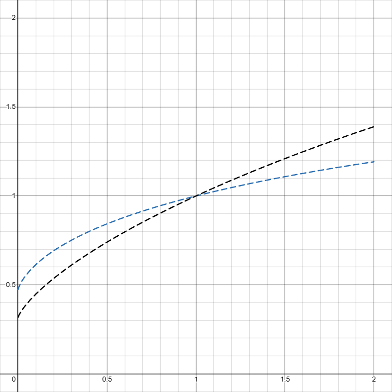
PDF scaled down to mean 1 \color{Blue}f(x), hazard function \color{Green}h(x):
If you don’t know what any of these means, here’s a brief explaination (mostly AI generated proof read by me, I learned all this in this project):
The hazard function, often denoted as h(t), describes the instantaneous risk of an event (like failure or death) happening at a precise time t, given that it has not occurred up to that time. In this case, it describes the propensity of the portal being lit at a certain point of time, given it was not lit before then.
In simpler terms, it answers the question:
“Given that you have survived (or not failed) until now, what is your immediate risk of failing right at this moment?”
Mathematically, it’s defined as the ratio of the probability density function(PDF) (here denoted as f(x)) (how likely failure is around time t) to the survival function (the probability of surviving past time t).
Key intuition:
- It’s not a probability; its value can be greater than 1.
- A constant hazard means risk doesn’t change over time (exponential distribution).
- Increasing hazard means aging/wear-out (e.g., machinery).
- Decreasing hazard means early risks that diminish (e.g., recovering after surgery).
There are very good reasons why \operatorname{arctan} works exceedingly well for predicting h(x). In a wood lighting process, the rate of portal lighting at start is lower(dependent on lava directly generating¹ fire in places that lights the portal), and gradually grows to a maximum rate(there can only be so much fire that speeds up the lighting process before it actually lights).
1. Wood Light Properties
Definitions
Under the pncakespoon wood light setup,
\color{Blue}{f(x)} is the probability density function of portal lighting at moment x and as a PDF naturally has \int_{0}^{\infty}f(x)dx = 1.
In the last chapter I standardized f(x) to mean 1, meaning m=\int_{0}^{\infty}xf(x)dx = 1, scaling down by a factor of S \approx 15.9149. Once we get the results under this, we can just use the same scale factor to scale back up.
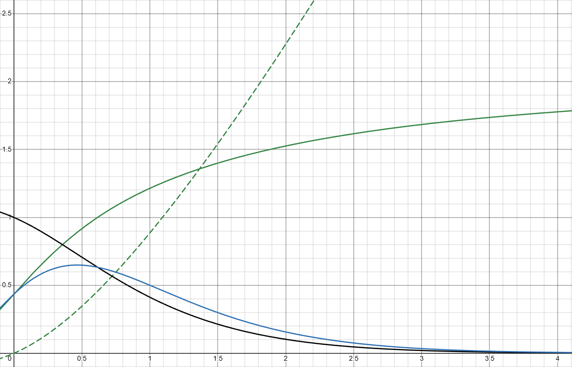
\color{Green}h(x)(solid) is the hazard function of portal lighting at moment x and has to meet \int_{0}^{\infty}h(x)dx = \infty, otherwise there will be a chance of portal never lighting.
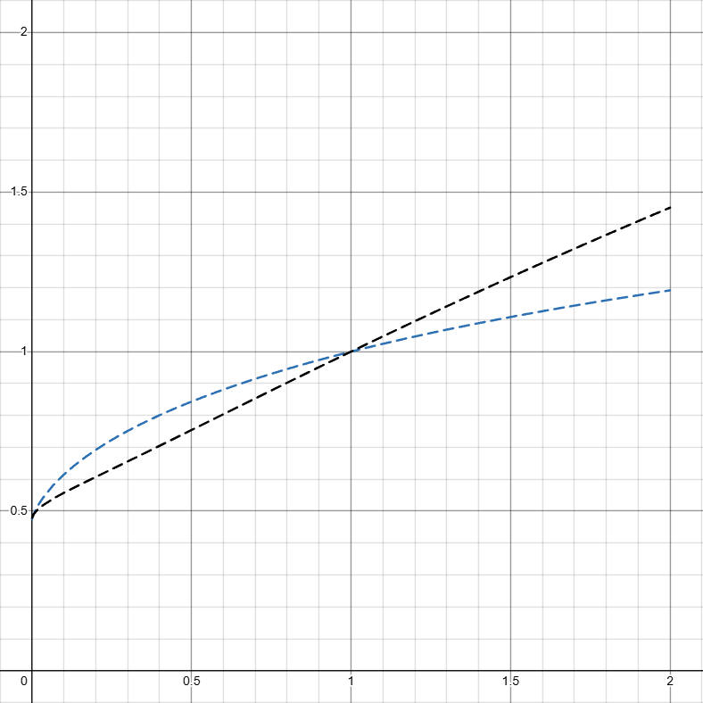
\color{Green}H(x)(dashed) is the cumulative hazard function, H(x)=\int_{0}^{x}h(y)dy.
\color{Gray}s(x) is the survival function of portal not lighting before moment x, s(x)=e^{-H(X)}.
h(x)=\frac{f(x)}{s(x)}.
Properties
If we have any other probability density function(for different setups, time acceleration rule, etc.) for portal lighting:
-
Under the same setup, any time acceleration rule must be normalized such that the probability density function of portal lighting f_a(x) generated under it also meets \int_{0}^{\infty}xf_a(x)dx = 1 (the average time that the portal being lit must not change, preventing any meta shifts between wood lighting and getting gravel).
-
Under the same time acceleration rule(not accelerating at all counts as a rule as well), the average time difference between setups(a good setup and a bad setup) should be preserved as well as possible. For simplicity, I set a ‘bad’ setup’s hazard function h_b(\delta,x) = \delta h(x), where \delta is a parameter to determine how bad the setup is.
Define m_b(\delta)=\int_{0}^{\infty}xf_b(\delta,x)dx , where
f_b(\delta,x)=h_b(\delta,x)s_b(\delta,x) , s_b(\delta,x)=e^{-\int_{0}^{\infty}h_b(\delta,x)dx},
We measure the deviation of average time difference
D(\delta) = \frac{\frac{m_b(\delta)}{m}}{\frac{1}{\delta}} = \delta\int_{0}^{\infty}x \delta h(x) e^{-\int_{0}^{\infty}\delta h(y)dy}dx = \delta^2 \int_{0}^{\infty}x h(x) e^{-\delta\int_{0}^{\infty} h(y)dy}dx :
-
Based off the two rules above, we minimize the luck factor (that is, the average time difference of two players doing the same benchmark setup). Here I use the time difference squared to ensure that it is positive, and also I argue losing 30s on wood light don’t just feels twice as bad as losing 15s, but 4 times as bad. In other words, we minimize C_{luck}=\int_{0}^{\infty}\int_{0}^{\infty}f(x)f(y)(x-y)^2dxdy, which for the pncakespoon wood light setup is \approx 1.1397.
2. Modeling & Solutions
Modeling
Define time acceleration kernal function k(x) to be the effective time warp rate for fire generation at moment x, and cumulative time passed function K(x)=\int_{0}^{x}k(y)dy.
The default time warp rate k(x)=1 and K(x)=\int_{0}^{x}1 dy=x.
Under the time acceleration kernal, define the cumulative hazard function H_k(x) = \int_{0}^{K(x)}h(y)dy , hazard function h_k(x) = H_k'(x), survival function s_k(x) = e^{-H_k(x)} , probability density function f_k(x)=h_k(x)s_k(x).
Just throwing in any random k(x) isn’t ever going to meet m_k = \int_{0}^{\infty}xf_k(x)dx = 1. In practice, I calculate m_{k_0} for the original k_0(x), then solve numerically the scale c_k such that when the kernal is k(x) = c_k k_0(x), m_k = 1. I will just call the pre-scale kernal function k_0(x) k(x) for simplicity.
In the desmos graph, instead of inputing k(x), I input directly K(x) to save an integral to speed up the calculation.
Solutions
Solution -1
If k(x)=1, meaning we have time flow at a normal rate, C_{luck} \approx 1.1397, and the average time difference across setups between normal time flow rate and normal time flow rate is literally 0.
Solution 0
Let k(x)=\{ x \leq c_{90}:1, x > c_{90}: 50\},
where \int_{0}^{c_{90}}f(x)dx = 0.9, meaning 90\% of time portal lights before c_{90} \approx 2.01767,
which is to say if the portal didn’t light before gS \approx 32.1110 seconds, we permanently crank up the time warp rate by 50 times before portal lights, which is basically forcing a light (edcr’s original solution). Here shows the comparison between \color{Blue}f(x) and \color{Gray}f_k(x) under k(x)=\{ x \leq c_{90}:1, x > c_{90}: 50\}:
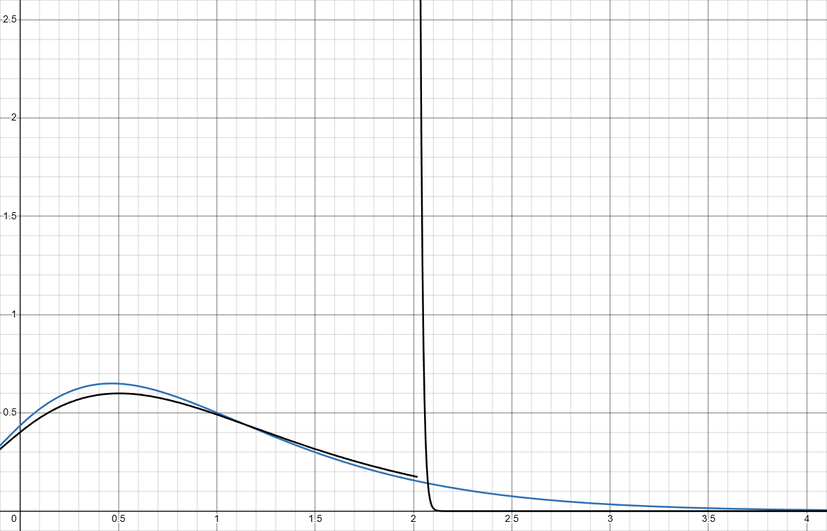
Note that \int_{0}^{c_{90}}f_k(x)dx \approx 0.8732 \neq 0.9 after the normalization for \int_{0}^{\infty}xf_k(x)dx = 1.
C_{luck}=\int_{0}^{\infty}\int_{0}^{\infty}f_k(x)f_k(y)(x-y)^2dxdy \approx 0.7874, which is a big improvement over 1.1397, but as I will show later there is a lot of room for improvement. The bigger issue however, comes from the deviation of average time difference over different setups compared to normal time flow rate.
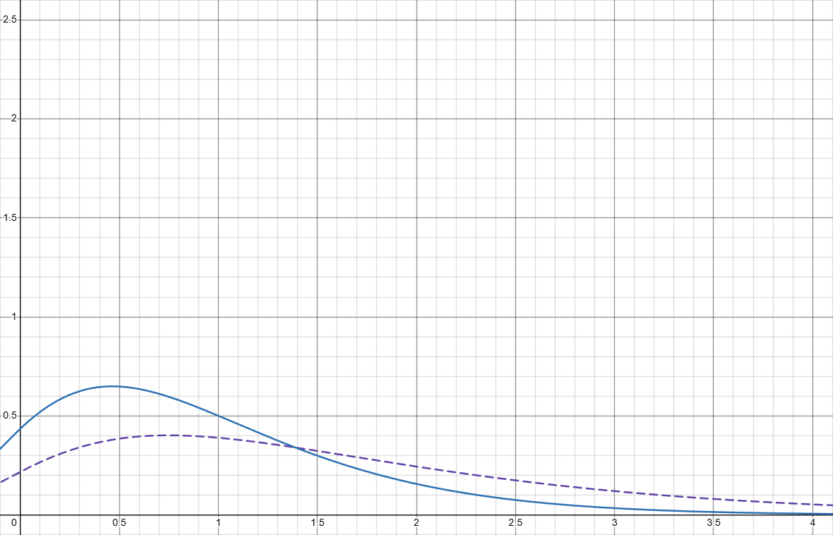
Here shows under k(x)=1, the comparison between \color{Blue}f(x) and \color{Purple}f_b(\delta,x) under \delta = 0.5:
And here is under k(x)=\{ x \leq c_{90}:1, x > c_{90}: 50\}, the comparison between \color{Gray}f_k(x) and \color{Orange}f_{kb}(\delta,x) under \delta = 0.5:
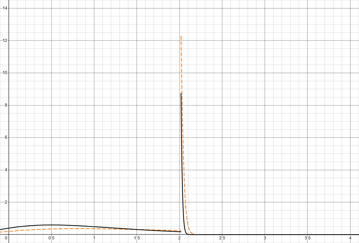
Intuitively you can tell that the worse wood light setup gets away more from the forced light at 32 seconds (all the tail after that gets squished on to a short period of time after 32 seconds). Measuring by \color{Blue}D(\delta) and \color{Gray}D_k(\delta), we can see the difference clearer (if you aren’t following, the two lines should be better closer together to show skill):
I did not squish the graph into a single scaler, not only because its debatable how much each \delta should matter, but also D(x) is incredibally slow to compute, the graph shown above is actually made by sampling 80 points and connecting them manually and it already takes like 15 seconds.
Solution 1
Let k(x)=ax+b, with a and b being hyperparameters, which is close to the solution in my mind when I proposed this solution in the original post. This means we start at a time warp rate slightly lower than 1 (after normalization, or else we can’t possibly have the mean m_k = 1 if k(x) > 1), then linearly speed up over time. Here shows the comparison between \color{Blue}f(x) and \color{Gray}f_k(x) under k(x)=x+1 (in red is normalized \color{Red}k(x) ):
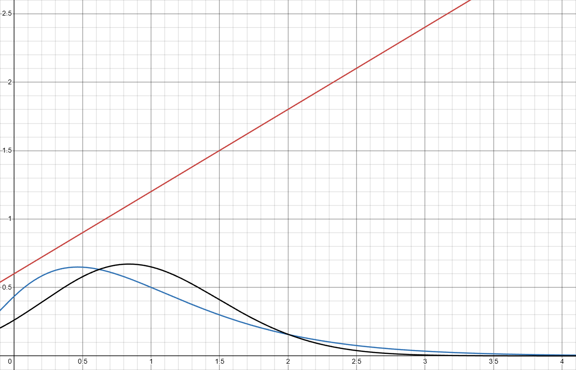
C_{luck} \approx 0.6574.
If you compare the two graphs, you can see there is a slight but not very drastic improvement on D_k(\delta) as well.
But we can do better than that.
Solution 2
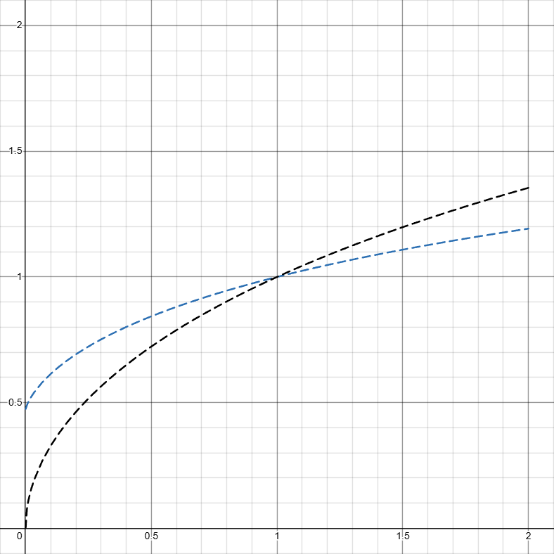
Let k(x)=\{ x \leq c:ax+b, x > c: ac+b\}. Here shows k(x)=\{ x \leq 1:2x+\frac{2}{3}, x > 1: 2+\frac{2}{3}\}:
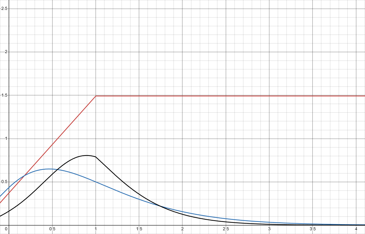
C_{luck} \approx 0.6191.
But in order to get the best C_{luck}, we can simply just have all the probability density concentrated at x=1 and we can achieve C_{luck} = 0. Where this solution really shines is D_k(\delta).
The part in x \leq 1 is infinitely better, though I would admit that the part after kind of blows up (nerfs carpet/leaf/flower light setup too much).
There must be even better k(x) families, that can max out on both scales. I suspect optimal k(x) is likely not even monotonic, and I will likely research for better k(x) later.
Data used are in:
26/01/09 Edit:
Extended D(x) graphs for wood light setups better than the benchmark setup(leaf, carpet, flower, etc.). Current solutions tends to nerf them a little too much which is concerning. I do believe there are k(x) families that can solve this and I am working on some solutions.
Also corrected a typo in the original post that the linear k(x) example showed is k(x) = x + 1 instead of k(x) = x + 2.
26/01/10 Note:
I ran a simulation with the pncakespoon setup but all the wood planks’ ignite and burn odds swapped into that of carpets(which is not even a feasible setup in game because it requires floating carpets), and got 14.29147 +- 0.15026 seconds, which is equivillant to \delta \approx 1.155, and it should be safe to say that is the absolute maximum we can realistically reach. And well, there is barely any deviation in the D(\delta) graph at \delta = 1.155 anyways so that should not be an issue.